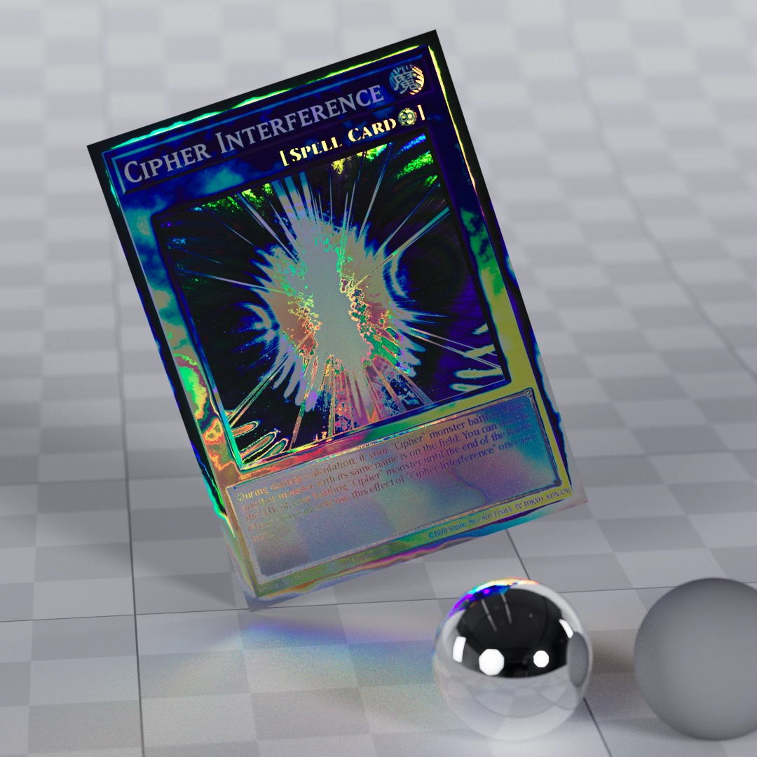
Appearance
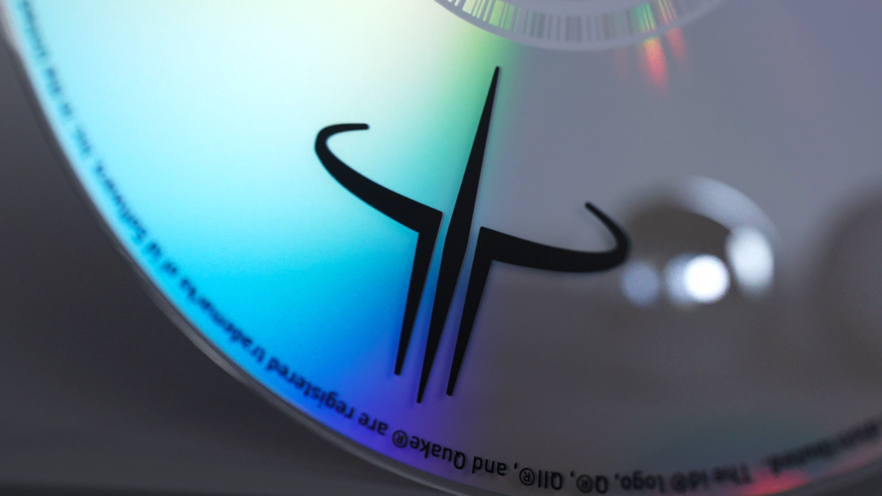
Diffraction grating is a wonderful but equally complex optical phenomenon. You've probably seen it on security holographic stickers, "holo" trading cards, and most commonly on optical disks.
The only realistic reproduction so far has been this OSL shader by Secrop, but it only works in Blender Cycles since Octane doesn't support OSL closures.
Ever since I found it, I became obsessed with reproducing the visual appearance of diffraction grating in Octane Render. It took many years, but I eventually managed to create a photorealistic method for holographic stickers and trading cards, as well as the rainbow effects seen on CDs and DVDs.
This guide shows how to simulate diffraction grating effects in Octane using physically-based rendering techniques. Rather than attempting to recreate the wave interference that causes real diffraction, this method combines light dispersion with microscopic surface geometry to achieve visually identical results, all rendered directly without compositing tricks or multiple passes.
Requirements
- Blender 4.5
- Octane Render 2025.1
How it works
Before we dive into the techniques, it's important to understand what we're actually recreating.
Real diffraction gratings work through wave interference. Light waves interact with nanometric periodic structures, and the waves interfere with each other to separate white light into its component wavelengths. This is a wave optics phenomenon that's extremely difficult to simulate in path tracers.
The method presented here doesn't attempt to simulate wave interference. Instead, it recreates the visual appearance of diffraction grating through a combination of:
- Dispersion: A refractive coating splits white light into colors, like a prism
- Microscopic geometry: Tiny periodic bumps on a reflective surface redirect light at specific angles
- Viewing angle dependency: Different angles see different wavelengths of the dispersed spectrum
The result is visually indistinguishable from real diffraction grating in most scenarios, achieved entirely through physically-based rendering without any compositing tricks. While the underlying physics differs from true wave interference, the visual output accurately matches what you'd see on holographic foils, trading cards, and optical disks.
Holographic foil
Let's start with the simplest effect: holographic foil. The key insight is that we need two components working together: a surface with microscopic directional geometry (to redirect reflections) and a dispersive medium (to split light into colors).
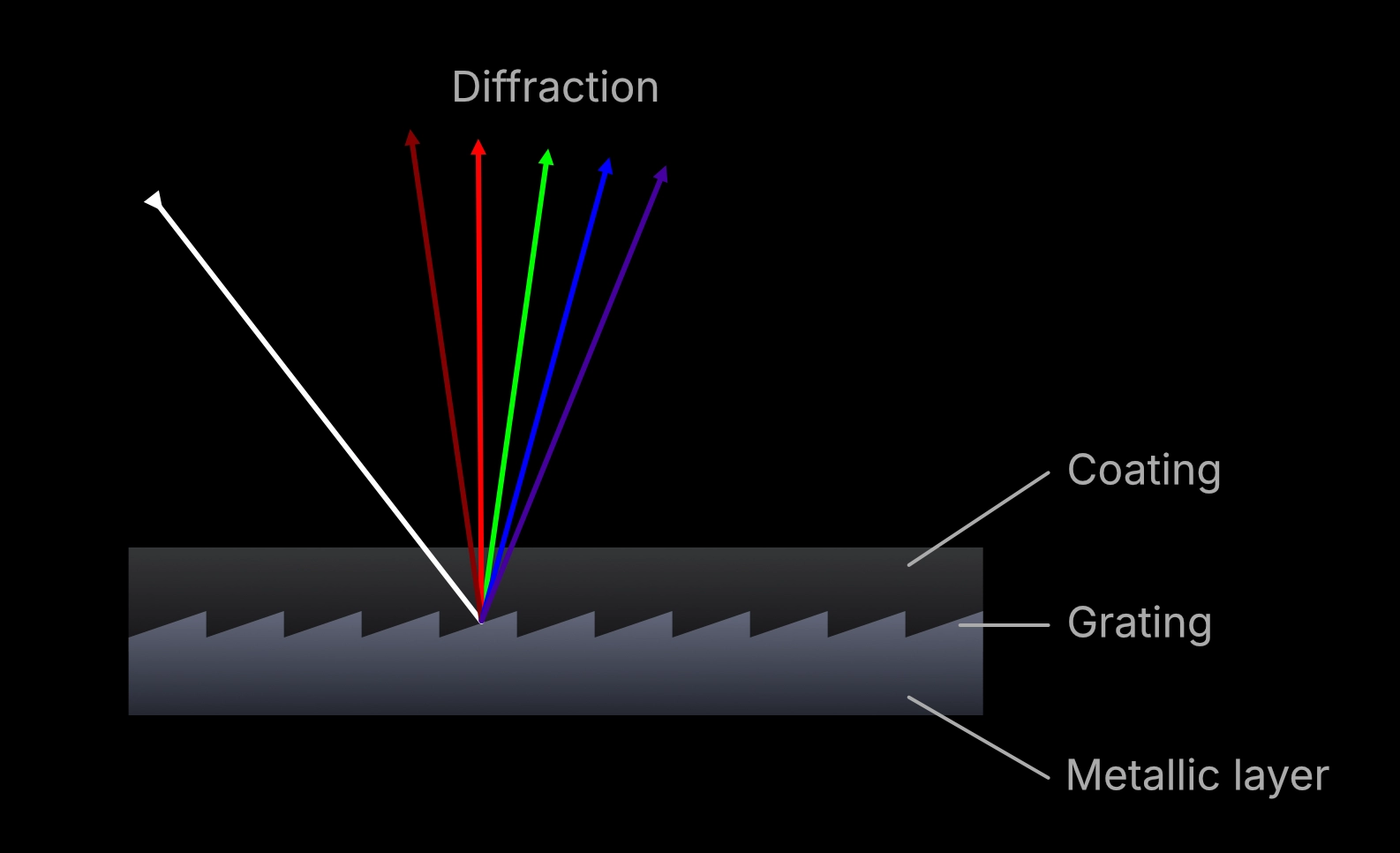
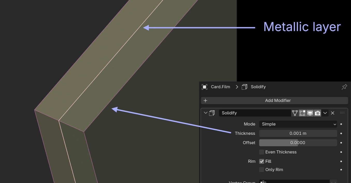
We'll need two very thin meshes: one metallic layer and one refractive coating.
Reflective layer
Create a plane and assign a new metallic material to it. Lower the roughness to zero so it behaves like a mirror.
Refractive coating
Duplicate the plane without changing its position. Apply a solidify modifier and set the thickness to 0.001 with the offset set to 0.0 (centered). This creates a solid[1] coating layer that envelops the metallic plane.
Apply a new specular material with the Reflection color set to pure black. Set the Dispersion Coefficient to any value greater than or equal to 1.0 and set the algorithm to Cauchy Formula.
Important
For the dispersion to be visible, use the Path Tracing, Photon Tracing or PMC kernel.
Normal map
In the specular material, set the reflective color to black, then connect the RGB color #8080FF to the normal input of the metallic material.
Position the camera at an angle to the plane to get a contrasty image in the reflection.
If you slightly change the red value of the normal map color (to say 0.51), you should see the dispersion of the reflected image.
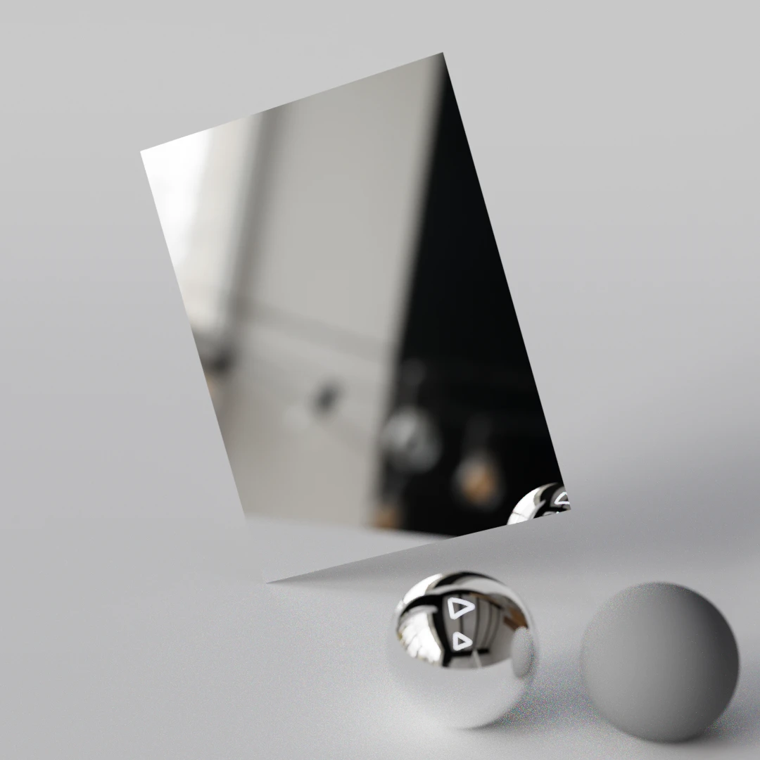

This is the foundation for all the effects I'll demonstrate in this guide.
What we've done is emulate a microscopic saw wave pattern seen from above on our metallic layer. The normal creates angled microfacets that redirect reflections, while the dispersive coating separates those reflections into spectral colors. When viewed from different angles, you see different parts of the dispersed spectrum, creating the characteristic rainbow effect associated with diffraction gratings.
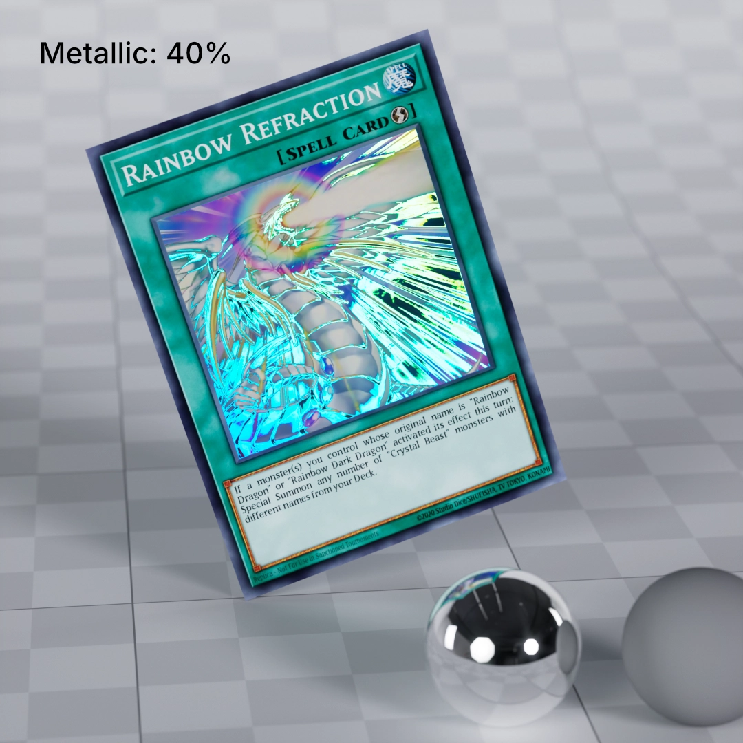
Trading card
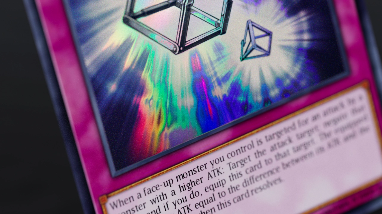
For this effect, we'll use an image texture to manipulate the shading normals of the metallic layer. This adds one level of complexity to our initial setup.
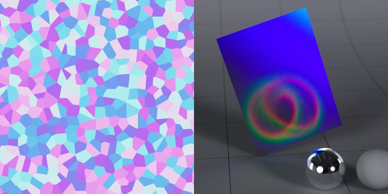
Create a Mix Texture node and use a grayscale image (linear gamma) for the amount. Set the two texture inputs to #C3BCFF and #C0B6FF, then plug the mix node into the normal input of the metallic material.

These are arbitrary normals represented as RGB colors. Any other normal would work, and you'll probably need to experiment with different ones to get a pleasing effect. Start from rgb(0.5, 0.5, 1.0) and adjust the red and green levels slightly.
By hiding and showing the refractive coating mesh, you can see how the normals in the underlying surface reflect different parts of the environment.

This is still rough, but clearly the right direction. The current node setup doesn't give us much flexibility, and it's difficult to find the right combination of colors to use in the normal map. We can only mix[2] between two angles, and we don't have much control over how the image texture affects the normals of the shader.
Microembossing OSL
To go further, we'll use OSL (Open Shading Language) textures to create the microembossed surfaces and gratings. OSL allows us to accurately create very fine and detailed maps without worrying about compression, resolution, or vRAM usage.
Right now we'll use OSL to accurately rotate the normal of our surface according to a grayscale texture. We specifically want to control the influence of the grayscale map on the rotation and the starting angle from which we rotate (Rotation Bias).
osl
// microemboss.osl
#include <octane-oslintrin.h>

shader Microemboss(
    point proj = point(u, v, 0) [[ string label = "Projection", string inputType = "projection:uvw" ]],
    matrix xform = 1 [[ string label = "UV transform", string type = "uvw" ]],
    color rotationMap = 0.0 [[ string label = "Rotation Map" ]],
    float rotationMapAmount = 360.0 [[ float min = 0.0, float max = 360.0, string label = "Rotation Map Amount (degrees)" ]],
    float rotation = 0.0 [[ float min = 0.0, float max = 360.0, string label = "Rotation Bias (degrees)" ]],
    float amplitude = 0.5 [[ float min = 0.0, float max = 2.0, string label = "Normal Amplitude" ]],
    output color C = color(0.5, 0.5, 1.0))
{
    point uvw = proj - point(0.5, 0.5, 0.0);
    uvw = transform(1/xform, uvw);

    float uu = uvw[0];
    float vv = uvw[1];

    // Evaluate rotation map texture input
    point projEval = transform(xform, point(uu, vv, 0)) + point(0.5, 0.5, 0.0);
    color rotMapValue = _evaluateDelayed(rotationMap, projEval[0], projEval[1]);

    // convert grayscale (rgb average) to rotation angle (0-1 -> 0-rotationMapAmount degrees)
    float mapRotation = (rotMapValue[0] + rotMapValue[1] + rotMapValue[2]) / 3.0 * rotationMapAmount;

    // add rotation bias
    float totalRotation = rotation + mapRotation;

    // convert to radians and calculate normal direction
    float angle = radians(totalRotation);

    // create a normal vector pointing in the rotation direction with given amplitude
    // the normal tilts in the direction specified by the angle
    vector nrm = normalize(vector(sin(angle) * amplitude, -cos(angle) * amplitude, 1.0));

    C = color(0.5 * (nrm[0] + 1.0), 0.5 * (nrm[1] + 1.0), 0.5 * (nrm[2] + 1.0));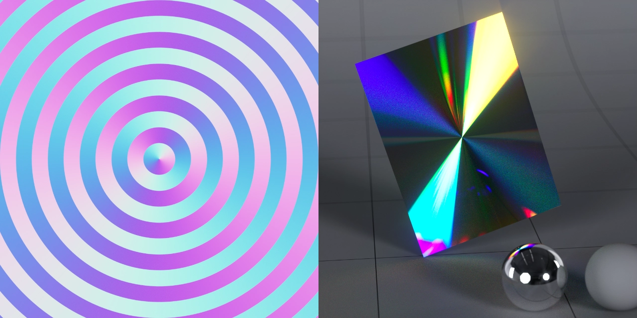
}We can test it by connecting an angular gradient. We should get a full 360 degree rotation, making a conic normal map at the output.
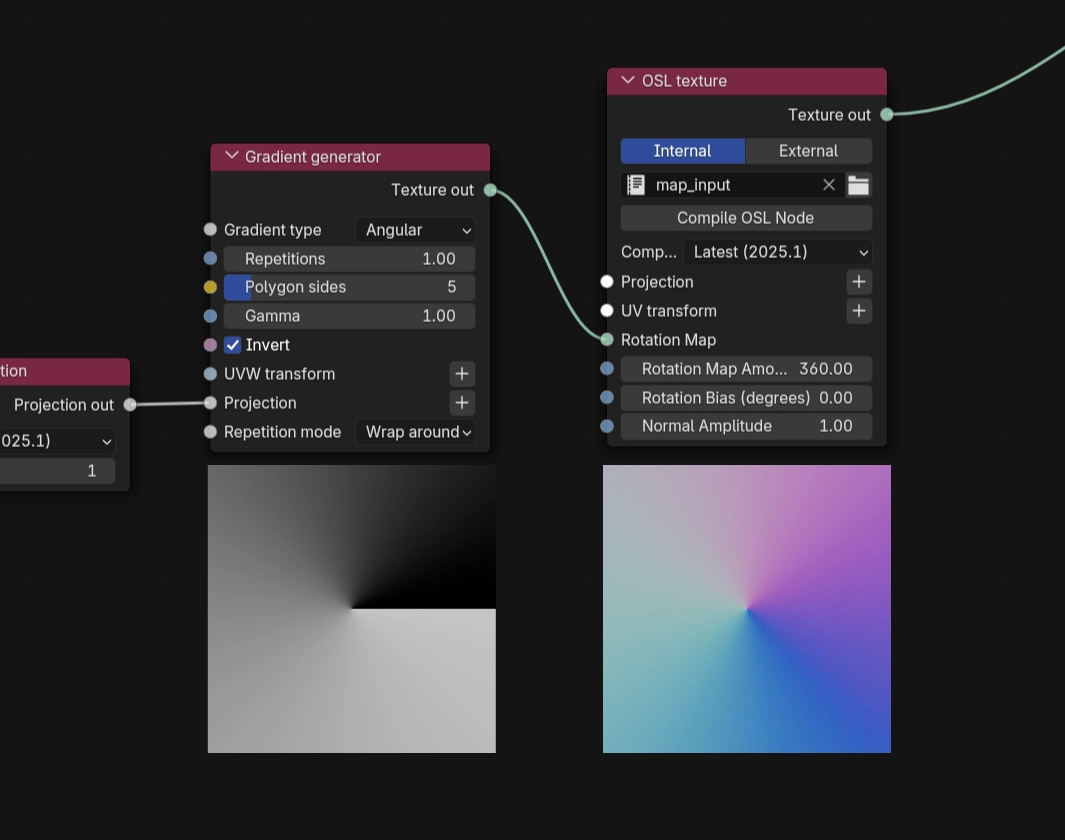
Note
We use the Gradient Generator just to visualize how the OSL script transforms grayscale colors. You should use your own linear grayscale image texture instead.
With a few tweaks to the material, we can now render realistic holographic effects on trading cards.
To localize the effect to only a certain area, use a Mix Texture node to set the normal map of the unaffected area of the card to #8080ff. The same areas of the inner mesh have been set to non-metallic with some specular roughness using a Universal Material.
So far we've used a pure metallic material as a base for the trading card, but non-metallic reflective materials work well too. For this shot, the Metallic parameter of the Universal Material has been set to 0.4 on the card's artwork. See Metallic vs Plastic base.
Although we haven't yet created the actual Grating in Diffraction Grating.
Update
For more control over the trading card shader, you can check out this node setup.
Microscopic Surface Geometry
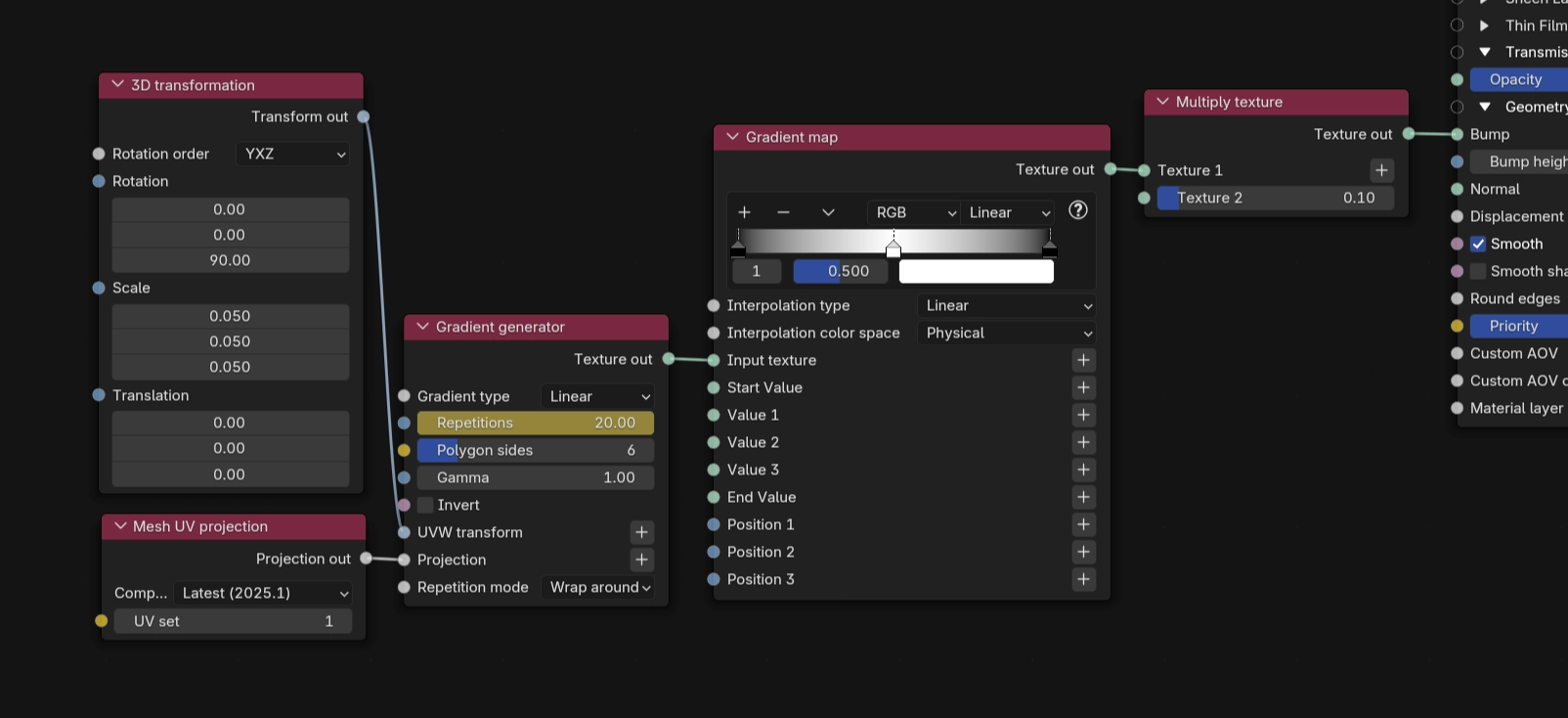
To simulate a real grating pattern, we need to create tiny regular structures on the metallic surface. These microscopic bumps will redirect reflections at controlled angles, which when combined with our dispersive coating, creates the characteristic spectral separation. To demonstrate the effect, we'll start with a procedural bump map.
Gradient Generator
Add a Gradient Generator node, set the type to Linear and the repetition to a high value. Make sure the Gamma is set to 1.0.
Triangle wave from saw
Since we want the bumps to reflect light at the same angle in both directions, we need to transform the saw wave into a triangle wave with the Gradient Map node. Add a new stop at 0.5 and set it to pure white, then change the final stop (at 1.0) to black.
This effectively changes the shape by moving the peak of the bump toward the center of the gradient while keeping the period unchanged.
TIP
This step is important because we want to see reflections from both sides when the surface is tilted at a steep angle. With the saw wave, we would see artifacts when tilting the surface at steep angles relative to the camera.
Adjust the scale
Depending on your mesh size, camera position, and environment, you might want to adjust the scale of the grating and the intensity of the effect.
Add a Scale Transform or 3D Transform node to the Gradient Generator, alongside a UV Mesh projection node. Scale down the grating until the lines aren't distinguishable anymore.
Then, before the bump input on the material, add a Multiply Texture node, set the second operand to 0.0, and slowly drag it up to a higher value.
By increasing and decreasing the scale or repetitions of the grating, you can see how the effect is created.
You might have noticed that changing the scale of the grating also changes the intensity of the effect (the reflected image stretches and compresses). This happens because with the same bump height, higher frequencies result in steeper angles.
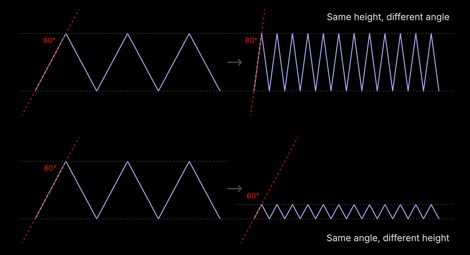
To compensate, the bump height from the Multiply Texture node has to be adjusted so that the height and frequency are inversely proportional to each other.
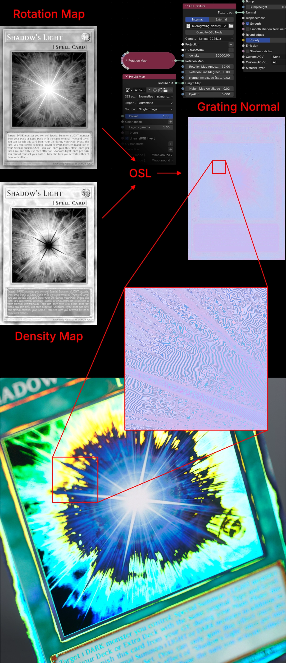
Grating OSL
Now that we know how to create a grating with a bump map, we can write an OSL script to generate a normal map with a triangle wave. This adds three important features:
- Angle compensation: The script decreases the height of the grating as density increases, maintaining the same angle on the microfacets.
- Rotation map: We can rotate the grating direction with a grayscale texture to create more visually complex diffraction grating examples.
- Height map: If needed, we can increase the steepness of the grating using a grayscale map. This changes the color reflected at the same camera-surface angle.
osl
// micrograting.osl
#include <octane-oslintrin.h>

shader Micrograting(
    point proj = point(u, v, 0) [[ string label = "Projection", string inputType = "projection" ]],
    matrix xform = 1 [[ string label = "UV transform", string type = "uvw" ]],
    float density = 1.0 [[ float min = 1.0, float max = 1e12, float sliderexponent = 3 ]],
    color rotationMap = 0.0 [[ string label = "Rotation Map" ]],
    float rotationMapAmount = 360.0 [[ float min = 0.0, float max = 360.0, string label = "Rotation Map Amount (degrees)" ]],
    float rotation = 0.0 [[ float min = 0.0, float max = 360.0, string label = "Rotation Bias (degrees)" ]],
    float amplitude = 0.5 [[ float min = 0.0, float max = 2.0, string label = "Normal Amplitude (Baseline)" ]],
    color heightMap = 0.0 [[ string label = "Height Map" ]],
    float heightMapAmplitude = 0.0 [[ float min = 0.0, float max = 2.0, string label = "Height Map Amplitude" ]],
    float eps = 1e-4 [[ string label = "Epsilon" ]],
    output color C = color(0.5, 0.5, 1.0))
{
    point uvw = transform(1/xform, proj - point(0.5, 0.5, 0.0));
    float uu = uvw[0];
    float vv = uvw[1];

    // evaluate rotation map and calculate total rotation
    point projEval = transform(xform, point(uu, vv, 0)) + point(0.5, 0.5, 0.0);
    color rotMapValue = _evaluateDelayed(rotationMap, projEval[0], projEval[1]);
    float mapRotation = (rotMapValue[0] + rotMapValue[1] + rotMapValue[2]) / 3.0 * rotationMapAmount;

    float angle = radians(rotation + mapRotation);
    float cos_a = cos(angle);
    float sin_a = sin(angle);

    // evaluate height map at center position
    color heightMapValue = _evaluateDelayed(heightMap, projEval[0], projEval[1]);
    float heightMapGray = (heightMapValue[0] + heightMapValue[1] + heightMapValue[2]) / 3.0;

    // calculate total amplitude: baseline + (heightMap * heightMapAmplitude)
    float totalAmplitude = amplitude + (heightMapGray * heightMapAmplitude);

    // scale amplitude inversely with density to maintain constant slope angle
    float scaledAmplitude = totalAmplitude / density;

    // helper function to calculate triangular wave value with per-sample amplitude
    float calculateWave(float uu_coord, float vv_coord) {
        // Evaluate height map for this specific position
        point sampleProj = transform(xform, point(uu_coord, vv_coord, 0)) + point(0.5, 0.5, 0.0);
        color hmValue = _evaluateDelayed(heightMap, sampleProj[0], sampleProj[1]);
        float hmGray = (hmValue[0] + hmValue[1] + hmValue[2]) / 3.0;

        // Calculate amplitude for this sample
        float sampleAmplitude = (amplitude + (hmGray * heightMapAmplitude)) / density;

        float uu_rot = uu_coord * cos_a - vv_coord * sin_a;
        float phase = mod(uu_rot * density, 1.0);

        // Simple triangular wave: rises 0->1 in first half, falls 1->0 in second half
        float wave = (phase < 0.5) ? (phase * 2.0) : (2.0 - phase * 2.0);

        return (wave * 2.0 - 1.0) * sampleAmplitude;
    }

    // calculate height at center and offset positions in UV space (not rotated space)
    float h = calculateWave(uu, vv);
    float h_dx = calculateWave(uu + eps, vv);
    float h_dy = calculateWave(uu, vv + eps);

    // calculate normal from tangent vectors in UV space
    vector dx = vector(eps, 0, h_dx - h);
    vector dy = vector(0, eps, h_dy - h);
    vector nrm = normalize(cross(dx, dy));

    C = color(0.5 * (nrm[0] + 1.0), 0.5 * (nrm[1] + 1.0), 0.5 * (nrm[2] + 1.0));
}We can now replace the bump-defined grating by plugging this script's output into the Normal input of the metallic layer in our scene. Now we have much more control over the angle of the generated grating, and we can change the density without having to manually adjust the height.
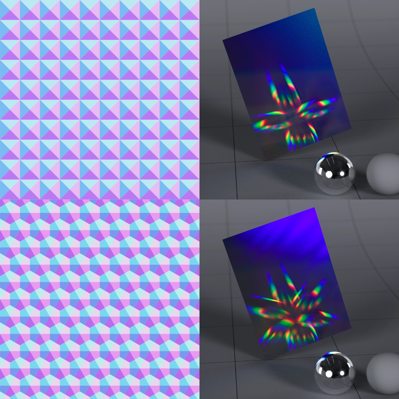
To visualize the functionality of this grating OSL script, we can feed a grayscale map into the Rotation Map input and observe how it responds when increasing the rotation amount and intensity.
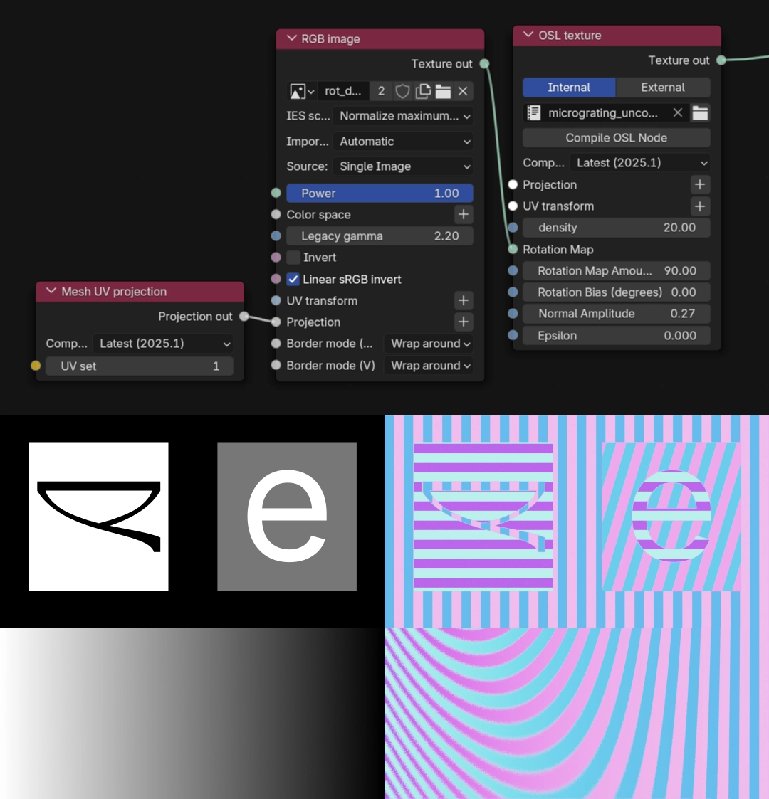
As a result, the grating in areas defined by pure black stays at the angle defined by Rotation Bias, while the map's pure white translates to a grating at the angle defined by Rotation Map Amount.
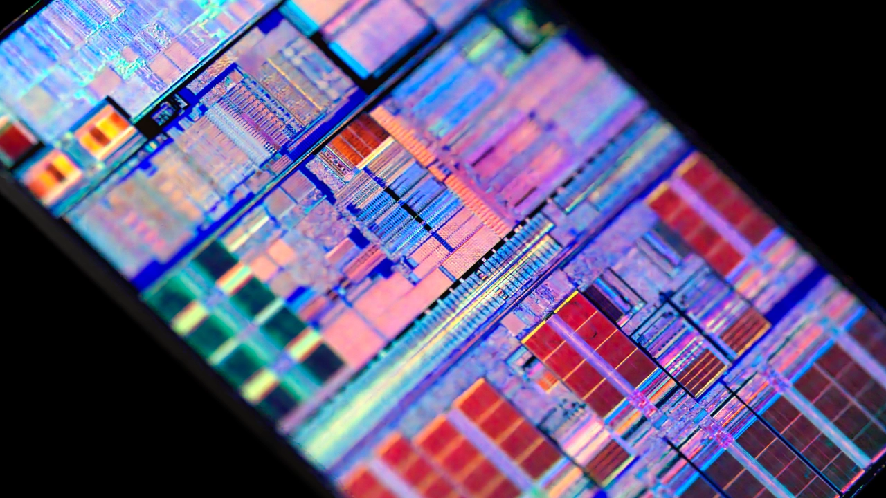
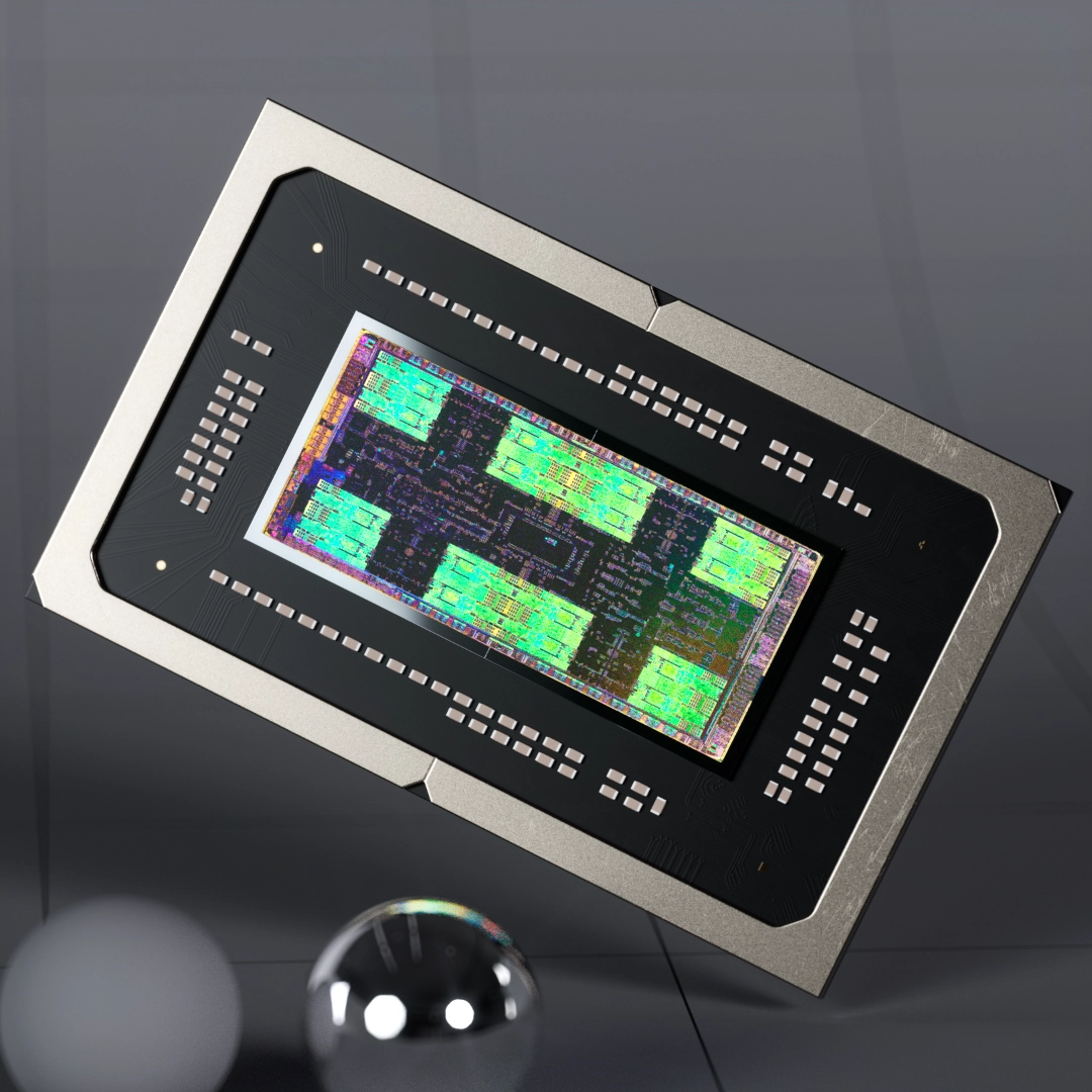
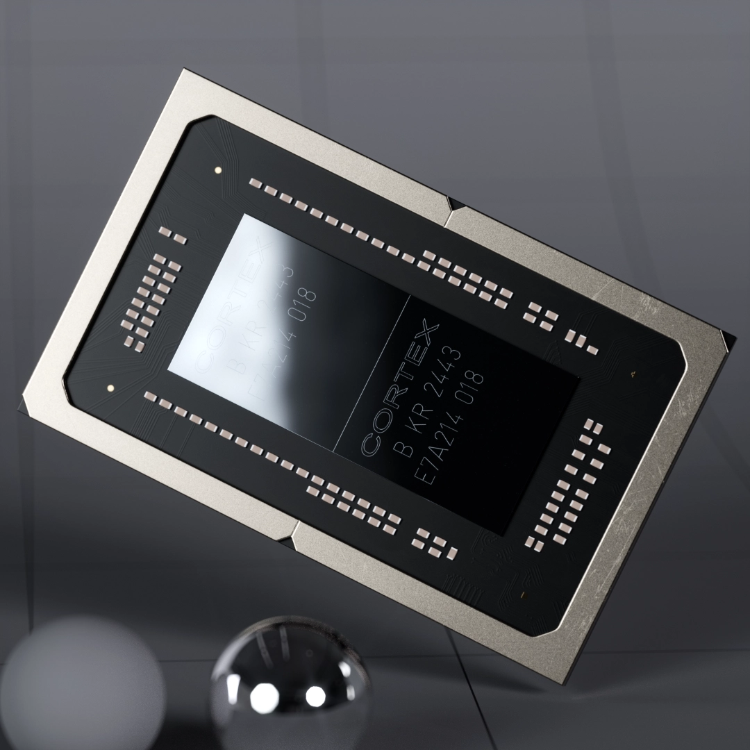
With this script, we can recreate the effect seen on CPU dies. The mesh setup is identical to the initial setup: a substrate layer with the grating shader normal and a thin dispersive layer that envelops the grating.
For this render, the grating material has been designed to mimic the visual properties of Silicon.
At this point, you might already have an idea of how the CD/DVD shader is achieved.
Optical Disk
For this effect, all we need is to tweak the micrograting.osl script that we used to create the anisotropic-like reflections for rendering the integrated circuit die.
For simplicity, we'll also get rid of the rotation controls of the microfacets, as CDs only have concentric grooves.
osl
// concentric.osl
shader ConcentricGrooves(
    point proj = point(u, v, 0) [[ string label = "Projection", string inputType = "projection:uvw" ]],
    matrix xform = 1 [[ string label = "UV transform", string type = "uvw" ]],
    float density = 1.0 [[ float min = 1.0, float max = 1e12, float sliderexponent = 3 ]],
    float amplitude = 0.5 [[ float min = 0.0, float max = 2.0 ]],
    float eps = 1e-4 [[ string label = "Epsilon" ]],
    output color C = color(0.5, 0.5, 1.0))
{
    point uvw = proj - point(0.5, 0.5, 0.0);
    uvw = transform(1/xform, uvw);

    float uu = uvw[0];
    float vv = uvw[1];

    float r = sqrt(uu*uu + vv*vv);
    float wave = abs(mod(r * density, 1.0) * 2.0 - 1.0) * 2.0 - 1.0;
    float h = wave * amplitude;

    float r_dx = sqrt((uu+eps)*(uu+eps) + vv*vv);
    float wave_dx = abs(mod(r_dx * density, 1.0) * 2.0 - 1.0) * 2.0 - 1.0;
    float h_dx = wave_dx * amplitude;

    float r_dy = sqrt(uu*uu + (vv+eps)*(vv+eps));
    float wave_dy = abs(mod(r_dy * density, 1.0) * 2.0 - 1.0) * 2.0 - 1.0;
    float h_dy = wave_dy * amplitude;

    // normalize the tangent vectors by density to maintain constant slope
    vector dx = vector(eps * density, 0, h_dx - h);
    vector dy = vector(0, eps * density, h_dy - h);
    vector nrm = normalize(cross(dx, dy));

    C = color(0.5 * (nrm[0] + 1.0), 0.5 * (nrm[1] + 1.0), 0.5 * (nrm[2] + 1.0));
}In most scenarios, you should be fine with Density values from 500 to 2000. In situations like closeups, you might find yourself needing to increase the grating Density parameter to make the individual grooves less noticeable. You may see that after a certain threshold (like a density above 10000), the effect reduces in intensity. This is where the Epsilon[3] parameter comes in handy. That control works just like Octane's Ray Epsilon setting, but for this OSL texture node only. Essentially, by reducing the Epsilon, you increase the resolution of the texture.
Tweaking the effect
By design, this effect produces a lot of color noise. For this reason, more samples are required for each frame. All the images and videos in this article have been rendered with sample counts from 500 to 1500, depending on the scene complexity.
You may also want to increase the value of Specular Depth depending on your scene. For example, adding a jewel case around the CD would require at least 24 samples in scenes I have tested.
Directed trading card grating
A more complex effect on the trading card can be achieved by using both the Rotation and Height map inputs of the script from the Microscopic Surface Geometry chapter.
The result differs from microembossing because gratings create bidirectional reflections (perpendicular to the groove direction), while microembossing creates unidirectional angled reflections.
In other words, we can rotate the anisotropic reflection that we see on the CD shader in directions defined by the input texture instead of having them in concentric circles.
The image below shows how two textures are used to modulate the angle and the height (or perceived density) of the grating, thus allowing us to control the anisotropic rotation and reflected wavelength.
Other surface features
You can enrich both the metallic layer (with the grating normal map) and the dispersive coating with additional material properties, such as bump maps (pictured below).

What about Roughness?
You might have noticed that all the renders above use glossy surfaces. This is because dispersion is only visible with smooth reflections. As roughness increases, the dispersed colors quickly mix into white noise.
To simulate a rough holographic surface, we cannot rely on Octane's Roughness control, as it randomizes light direction too much. Instead, we need controlled randomness that maintains a consistent viewing angle with the camera to prevent the dispersion from becoming white.
Pictured below is an OSL script that generates voronoi cell noise. Each cell maintains the same angle with the camera's Z axis, but the X and Y normals vary randomly within each cell.
This controlled variation allows us to create more diffuse holographic effects while preserving visible color separation. The same principle of orienting microscopic structures applies to the radial grooves in the CD shader.
We can also create more regular diffraction patterns often seen on mobile phone LCD screens. Using microscopic pyramidal bumps in the normal map, the base shape of each pyramid determines the number and arrangement of reflected images.
Metallic vs Plastic base
Trading cards often feature metalized surfaces. Setting the shader that features the embossing or grating normals to have metallic properties usually increases the realism.
Silicon Material
The following properties have been used in the image below and in the chip die video:
| Property | Value |
|---|---|
| IOR | 3.89, 4.16, 4.58 |
| Metallic reflection mode | RGB IOR |
| Metallic | 1.0 |
| Roughness | 0.0 |
| Normal | Grating OSL |
Silicon is not a metal, but in real life it has metallic-like reflections. Specifically, the reflections are tinted, so setting the Metallic value to 1.0 produces a realistic silicon material.
Previous work
There are many techniques online that attempt to reproduce this visual effect. Many seem realistic at first, but most rely on workarounds that don't hold up under scrutiny or in motion.
The most clever method has been published by Raphael Rau. It consists of manually separating the RGB components of the reflected light, technically creating diffraction "by hand."
Drawbacks
This method is by far the closest to being physically plausible, as the scene lights actually reflect on the object's surface and undergo some form of separation.
But the approach only separates red, green, and blue channels. A real spectrum contains yellow, orange, cyan, violet, and countless other wavelengths that won't appear in a simple RGB separation. The result can look convincing but lacks the full richness of true spectral dispersion.
Conclusion
This technique took years of experimentation to develop. While researching existing methods, I realized that most approaches either relied on compositing tricks or couldn't handle dynamic lighting and camera movement convincingly. I wanted something that would work entirely within the renderer, responding naturally to scene lights and viewing angles.
The solution combines dispersion through a refractive coating with carefully controlled microscopic surface geometry. It's not true wave interference, but it produces results that are visually indistinguishable from real diffraction gratings in nearly all practical scenarios. The dispersive coating handles the spectral separation that path tracers can actually simulate, while the geometric approach gives us precise control over the intensity and the anisotropic effect at each viewing angle.
What makes this method special is that it's entirely physically-based. No baked textures, no compositing passes, no HDRI tricks. Just light, geometry, and refraction working together the way they would in reality, albeit through a different physical mechanism than actual diffraction.
I'm sharing this openly because techniques like this shouldn't be gatekept. The OSL scripts, node setups, and underlying principles are yours to use, modify, and build upon. If you create something with this method or discover improvements, I'd love to see it.
We need this to be a solid mesh for the light to disperse realistically ↩︎
We are combining two normals in RGB space, but we should be gradually rotating the normal in XYZ space instead ↩︎
Resolution is controllable through the Epsilon parameter in the OSL scripts. By reducing the Epsilon value, the sampling resolution of the normal map increases. ↩︎